Telecom Paris Dep. Informatique & Réseaux Nils Holzenberger ← Home page February 2024

Neuro-Symbolic Artificial Intelligence

with

Simon Coumes

and

Zacchary Sadeddine

➜            other AI courses

When Alan Turing imagined the future of computer science in 1950, he saw clever machines able to learn as human children do. Now we know that this great scientist was somewhat naive on that issue. Learning has long been understood as mere statistical recording, in the spirit of empiricist philosophy, so Turing did not see the problem. Learning is now understood to require a relevance criterion saying what the system should pay attention to, what it should keep in memory and what it should ignore. Mere frequency often proves insufficient as relevance criterion. This is where complexity (next week topic) will come into play.

Both machine learning and complexity constitute vast domains. I only picked a few topics that are, to my view, relevant to this course. Readers are invited to dive deeper into these fascinating areas by themselves.

Reinforcement learning is halfway between symbolic and numerical learning techniques. It perfoms statistical computations on a set of symbolic states. This technique can be dramatically efficient on some occasions. Let us consider the Nim problem, as popularized in famous scenes of Alain Resnais’s well-known and surprising film, L’année dernière à Marienbad (you may watch the the excerpt, which includes the match game). In this game, players may take as many items from a single row in turn (in the figure below, items are matches, not cards). The one who takes the last item looses.

I wrote a small programme that implements a basic version of reinforcement learning. The idea is to store various states in memory, with a positive score when the state has been visited by the winner, and a negative score for states visited by the looser. Then, when playing, the machine tries to reach positively valued states while avoiding negatively valued ones. Inspect the program. Take a while to understand its structure.

Play a few games with the programme by typing the command game.
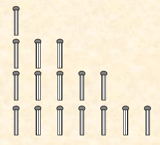
Observe that if you adopt the same behaviour twice, the machine tries to innovate to avoid making the same errors twice. If you are a perfect player (perfect players do exist in Nim games), then the machine will soon learn to be a match for you. You’ll probably lack the patience to teach it that far.

As I was still a student (some times ago!), I implemented this game as one of my first programs (yes, computers did exist at that time!) My initial idea was to have the program learn against a random player. This was the time when ideas like ‘noise a source of order’ (Edgar Morin, Henri Atlan...) were prevailing. The result proved miserable in that case. Random agents are too poor players to learn from. After several days of intense thinking, a brilliant idea occurred to me (a pity that most students come upon the same idea instantaneously when I tell the story): let’s have the programme play against itself!

This kind of technique has been implemented, in a less trivial way, by Gerald Tesauro who applied it to the Backgammon game (Jaquet, in French). His programme played at a master level and is said to have won a world contest in 1995. The number of possible states was too large for a machine to memorize them all. Therefore Tesauro used a neural network to classify states and work on classes instead.

More recently, using similar techniques, the Alphago program suceeded in beating a world champion in a game considered to be beyond current machines’ reach, Go.

Reinforcement learning introduces various refinements, such as a propagation of valuation (when a state proves interesting, all states that lead to it inherit part of that interest).

Reinforcement learning is a statistical learning method that takes advantage from the existence of a topology between states and from their frequency of visit. Statistical learning has many applications in data mining, text mining, corpus-based NLP, diagnostic, decision making, pattern recognition, spam detection, robotics, and so on. Many different techniques rely on statistical regularity:

• neural networks, deep learning
• self-organizing maps
• reinforcement learning
• clustering techniques
• support vector machines
• Bayesian networks
• decision trees
• genetic algorithms
• ... ... ...

Human learning quite often does not rely on statistics. Human children learn some ten new words a day during ten years. The meaning of most of these words is understood and memorized after a single occurrence (we know it from the relatively rare cases in which children misunderstand a word). Even in adulthood, unique (but highly relevant) situations may be remembered for life.
Human learning, contrary to statistical learning, is sensitive to structure. In what follows, we concentrate on the problem of structure, as it may be the major challenge of future machine learning.

Consider the two following instances of an unknown concept X (this example is borrowed from Ganascia, J-G. (1987). AGAPE: De l’appariement structurel à l’apprentissage. Intellectica, 2/3, 6-27).

These two examples can be described as:

E1 = square(A) & circle(B) & above(A, B)

E2 = triangle(C) & square(D) & above(C, D)

Now you want to guess what X is. Some candidates are: ‘anything’, ‘any group of geometric shapes’, ‘any group of two geometric shapes’, ‘any group of two geometric shapes involving a square’, ... One would obviously reject definitions that, though covering both examples, are too general. ‘any group of two geometric shapes’ looks better than ‘any group of geometric shapes’ because it is less general and still matched the two examples. The rule of induction reads:

Abstract the least general generalization (lgg) from the examples

(we’ll see below how this rule can be improved). One can see here the crucial role played by structure in concept learning. Another crucial ingredient of generalization is the possibility of using some background knowledge, such as the shape hierarchy pictured here.

The program lgg.pl aims at performing structural matching by looking for compatible features between two examples. Take a while to examine the program. Locate predicate matchTest at the end. It is used to test the program. It calls generalize, which calls match. Then match calls a predicate that you are supposed to write: lgg. When two features are not directly unifiable, lgg climbs up the shape hierarchy as necessary, until a match is eventually found. For instance, square(A) and triangle(B) cannot be unified at first, but a match is eventually found as both shapes satisfy polygon(_).
Note that feature structures are "executed" once unified. This is supposed to mimic perception. The effect is to instanciate shapes to actuals objects (named object_1 and object_2).

Much scientific work has been devoted during the seventies and the eighties to modelling symbolic induction using structural matching. This various attempts have been unified into a technique known as Inductive Logic Programming. As illustrated by the preceding exercise, the point of ILP is to perform a loose version of unification: square(A) and triangle(B) do not match, but they do unify if one accepts to generalize them a little bit. Note that the use of background knowledge (here, our small geometrical ontology) is crucial here. Let’s take another example (adpated from Buntime, W. (1988). Generalised subsumption and its applications to induction and redundancy. Artificial Intelligence, 36 (2), 149-176). Suppose we want to generalize the concept cute from the following two examples:

cute(X) :- dog(X), small(X), fluffy(X).        (1)
cute(X) :- cat(X), fluffy(X).                (2)

To match these two examples, we must drop most of the features. We get:

cute(X) :- fluffy(X).

which might be too general a conclusion. Can be use background knowledge to do better?
Consider the following knowledge:

    pet(X) :- dog(X).        (3)
    pet(X) :- cat(X).        (4)

    small(X) :- cat(X).        (5)

When properly used, this knowledge may lead to the following generalization:

cute(X) :- pet(X), small(X), fluffy(X).    (6)

which is less general, and thus better, than the initial one. A technique known as inverse resolution does exactly that. First, observe that resolution of (6) with (3) gives (1):
(6) corresponds to the clause: [cute(X), ¬pet(X), ¬small(X), ¬fluffy(X)]
(3) corresponds to the clause: [pet(X), ¬dog(X)]
As we can see, resolution between (6) and (3) gives: [cute(X), ¬dog(X), ¬small(X), ¬fluffy(X)] which, indeed, corresponds to (1).

Similarly, the resolution of (6) with (4) and then with (5) gives (2). The point of inverse resolution, as implemented in the programme Progol, is to get (6) from (1)+(3) and again from (2)+(4)+(5).

Finding efficient implementations of inverse resolution that may scale up is ongoing research.

We can see from the previous examples that background knowledge is crucial for efficient symbolic learning. It may explain why children (and also adults) are so good when learning new concepts, even from one single exposure.
In 1998, as I attended a conference in Göteborg, I was given the following object during the evening cheese & wine reception.

One could instantaneously tell who was Swedish and who wasn’t in the room. A Swedish delegate would clip the device on the plate, so that it could support her glass, allowing her to enjoy a spare hand to use a fork. No need for statistics here to get the point, and indeed I never forgot the concept. Moreover, I instantaneously understood that the blue ornaments (almost erased on the image) were irrelevant, whereas the opening in the circle was crucial. Of course, such learning feat is only possible because one knows much about the world of cocktail parties (that one usually needs three hands, that glasses should remain vertical, that gravity pull objects towards ground, ...).

Consider the following background knowledge.

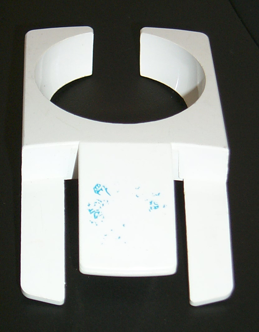
telephone(T) :- connected(T), partOf(T, D), dialingDevice(D), emitsSound(T).

connected(X) :- hasWire(X, W), attached(W, wall).
connected(X) :- feature(X, bluetooth).
connected(X) :- feature(X, wifi).
connected(X) :- partOf(X, A), antenna(A), hasProtocol(X, gsm).

dialingDevice(DD) :- rotaryDial(DD).
dialingDevice(DD) :- frequencyDial(DD).
dialingDevice(DD) :- touchScreen(DD), hasSoftware(DD, DS), dialingSoftware(DS).

emitsSound(P) :- hasHP(P).
emitsSound(P) :- feature(P, bluetooth).

Now, an example is given through a list of particular features:

example(myphone, Features) :-
    Features = [silver(myphone),
                belongs(myphone, jld),
                partOf(myphone, tc), touchScreen(tc),
                partOf(myphone, a), antenna(a),
                hasSoftware(tc, s1), game(s1),
                hasSoftware(tc, s2), dialingSoftware(s2),
                feature(myphone,wifi),
                feature(myphone,bluetooth),
                hasProtocol(myphone, gsm),
                beautiful(myphone)].

This particular object can be proven to be a telephone, using the above background knowledge. Some features, such as silver(myphone) turn out to be irrelevant to the proof.

The program ebg.pl contains the background knowledge and the description of the example. It also includes a prover, prove, that prints what it does.

From the trace collected when proving telephone(myphone), we can define a new concept:

C001(X) :- feature(X, bluetooth), partOf(X, Y), touchScreen(Y), hasSoftware(Y, Z), dialingSoftware(Z).

This definition has been obtained by generalizing shared constants within the trace. We may dig deeper into the structure of the trace and group together predicates that do not depend on X:

C002(Y) :- touchScreen(Y), hasSoftware(Y, Z), dialingSoftware(Z).

Now, the definition of C001 reads:

C001(X) :- feature(X, bluetooth), partOf(X, Y), C002(Y).

You can see how much can be learned from a single example (note that since the example leads to several alternative traces, even more can be learned). The new concepts are specializations of already known concepts, obtained through a generalization of particular objects (constants).

This situation contrasts with statistical learning, as used in neural networks or in standard clustering techniques. Statistical learning works on "flat" structures (typically numerical feature vectors). It is unable to take advantage of background knowledge and to perform the kind of structural learning achieved through ILP or EBG. The converse is not true: ILP or EBG may be supplemented to take statistics into account.

Though a combination of statistical and symbolic learning might represent the future of machine learning, several problems lie in the path leading to the autonomous learning machine Alan Turing dreamt of. The two main difficulties are the risk of combinatorial explosion that still limits the applicability of ILP, and the absence of predefined predicates in real life applications. For instance, in biological applications of machine learning, relevant structures that may explain protein chemical affinity are not known in advance.

The mathematical concept of complexity is likely to be a crucial conceptual tool that will be of great help to solve these problems. It will be studied in the next topic.

            

Back to the main page