Understanding Artificial Intelligence
through Algorithmic Information Theory
Prototype based models
and compression
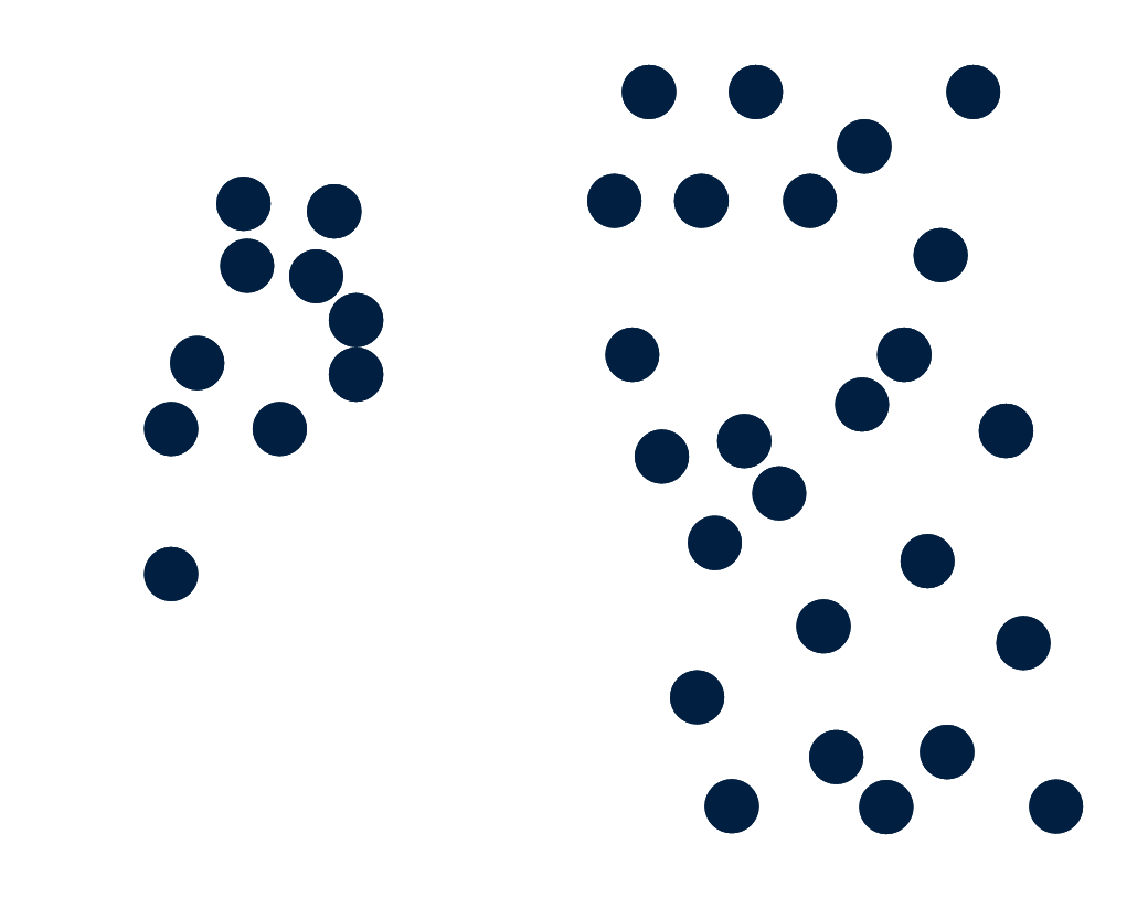 Prototype-based models
 can be used in unsupervised learning to group similar data points together (e.g. in marketing or recommender systems).
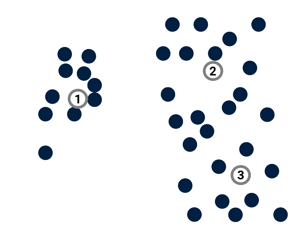 Prototype-based models
 can be used in unsupervised learning to group similar data points together.A prototype is a point of the input space used to provide information about the distribution of data points.
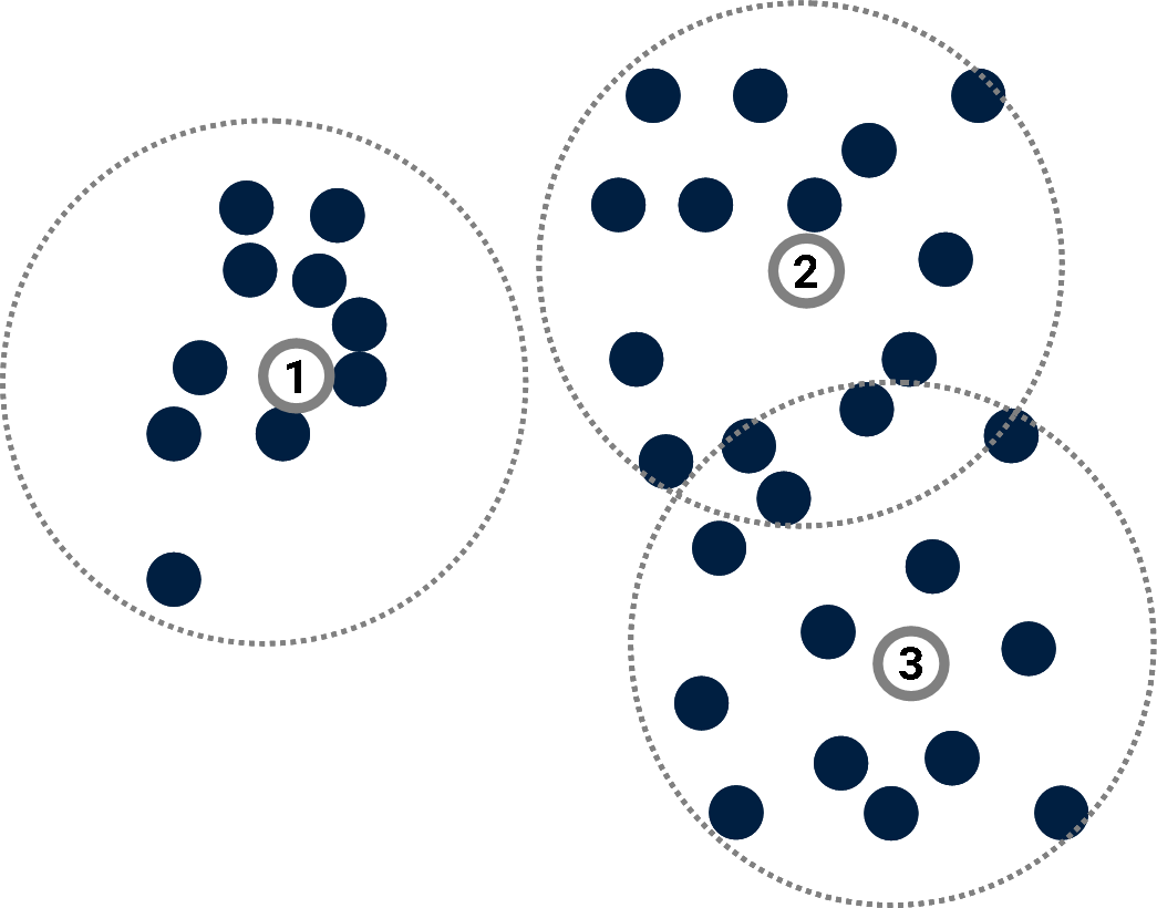 Prototype-based models
 can be used in unsupervised learning to group similar data points together.A prototype is a point of the input space used to provide information about the distribution of data points. Intuitively, data are distributed "around" the prototypes.
Prototypes models
One of the most famous prototype-based methods in machine learning is the K-Means algorithm.
Several improvements have been proposed (Learning Vector Quantization, Online Learning Vector Quantization, Self-Organizing Maps, Neural Gas algorithms, etc.).
Prototypes models
One of the most famous prototype-based methods in machine learning is the K-Means algorithm. You can watch nice Neural Gas demos

|
here |
|
|
and there |
 Compression
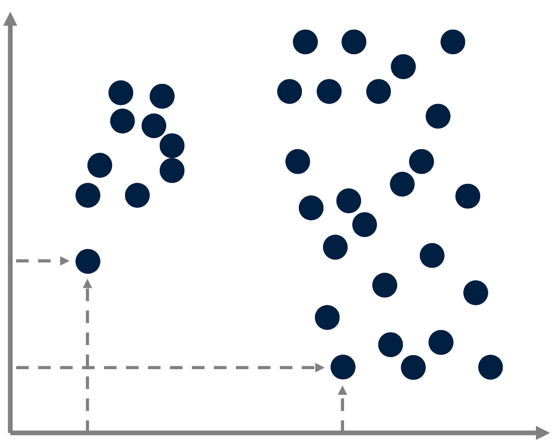
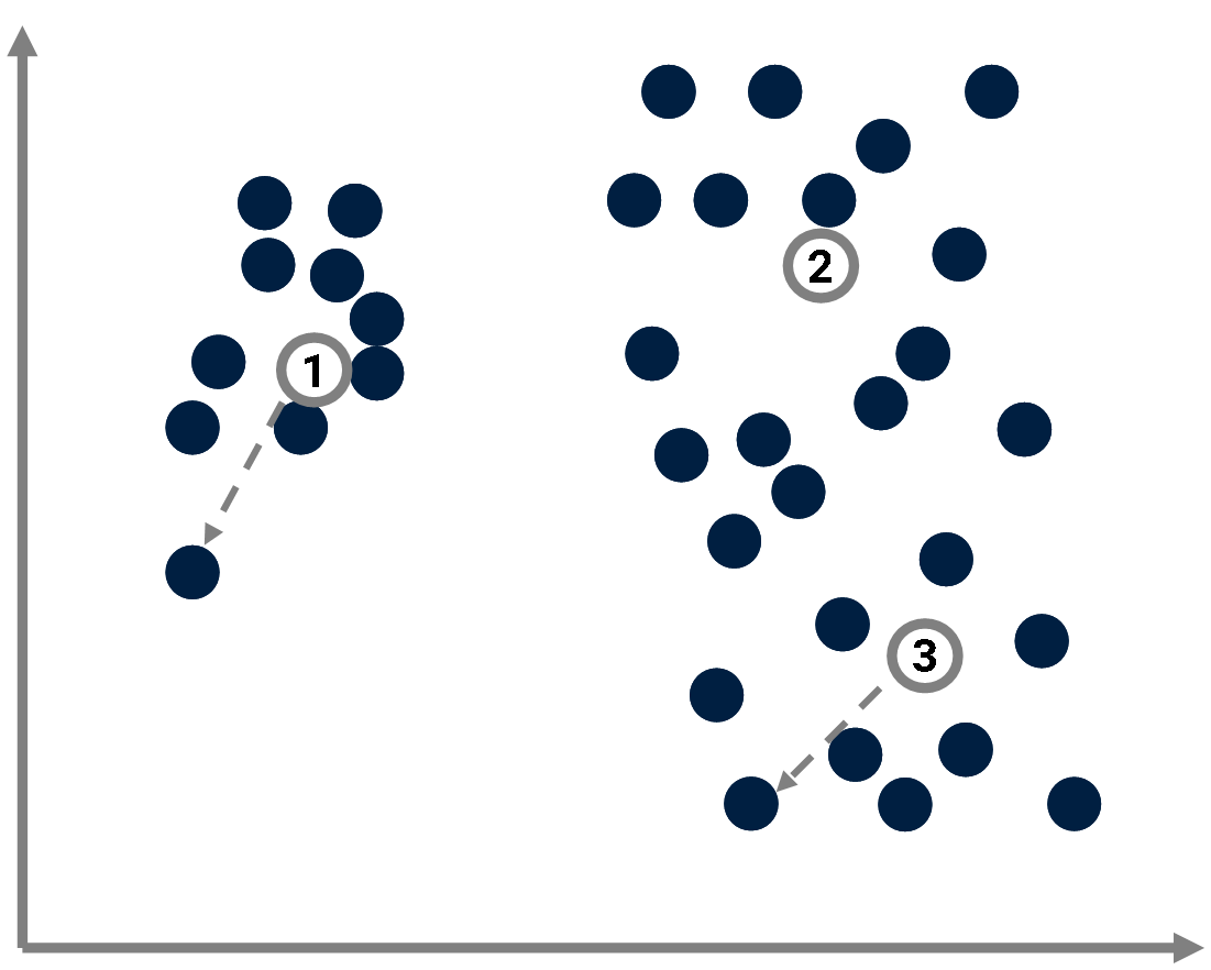
Prototype-based models can be seen as compression methods: Instead of describing data points by specifying their absolute coordinates,
 Compression
Prototype-based models can be seen as compression methods: Instead of describing data points by specifying their absolute coordinates,
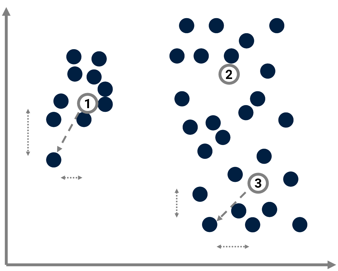
one considers their coordinates relative to the closest prototype.
 Compression
Prototype-based models can be seen as compression methods: Instead of describing data points by specifying their absolute coordinates,
one considers their coordinates relative to the closest prototype. We get smaller numbers, hence the compression.
Compression
The complexity of a point \(x_j\) in the dataset \(X\) is bounded by the complexity of its coordinates \((x_{j_1}, \dotsc, x_{j_d})\):
$$ C(x_j) \leq C(x_{j_1}) + \dotsc + C(x_{j_d}).$$
where the complexity of coordinates depends on the precision \(\delta\) used to convert them into integers.
We get a "naive" upper bound of the complexity of the whole dataset \(X\): $$C(X) \leq \sum_j C(x_j).$$
Compression
If prototypes \(\{p_k\}\) are introduced,
the complexity of \(X\) is now:
$$ C(X) \leq \sum_k C(p_k) + \sum_i C(x_j|\{p_k\})$$
where:
\(C(x_j|\{p_k\}) = \min_k C(x_j-p_k).\)
If the dataset exhibits some structure, suitable prototypes can be found and this estimate of \(C(X)\) will turn out to be significantly smaller that the "naive" one (hence the compression).
Conversely, and quite remarkably, this expression can be used to find the best prototype set \(\{p_k\}\)
(Cilibrasi & Vitányi, 2005). Classification
Now consider a classification task as an example of supervised learning.
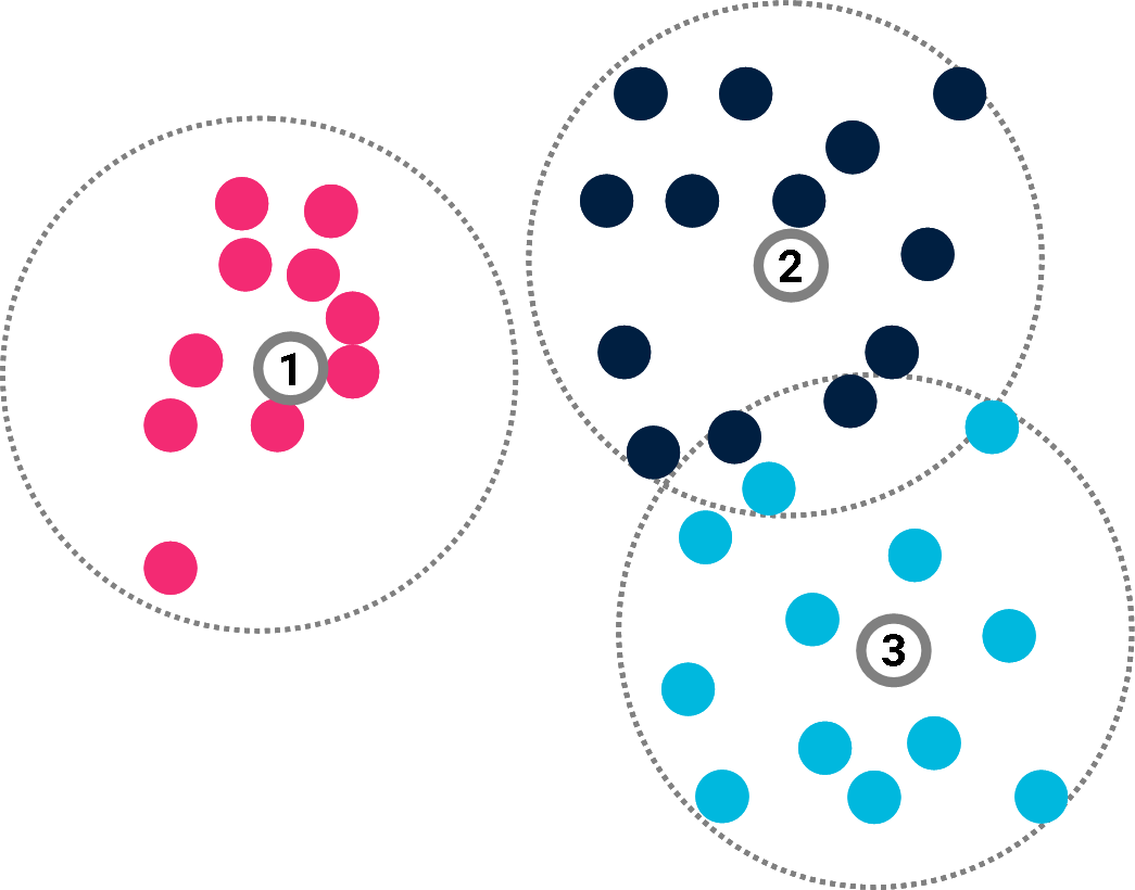
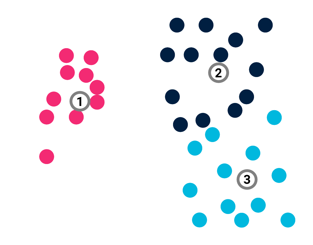
The problem is to associate a label (e.g. blue/red/dark) to each data point.
 Classification
Now consider a classification task as an example of supervised learning.
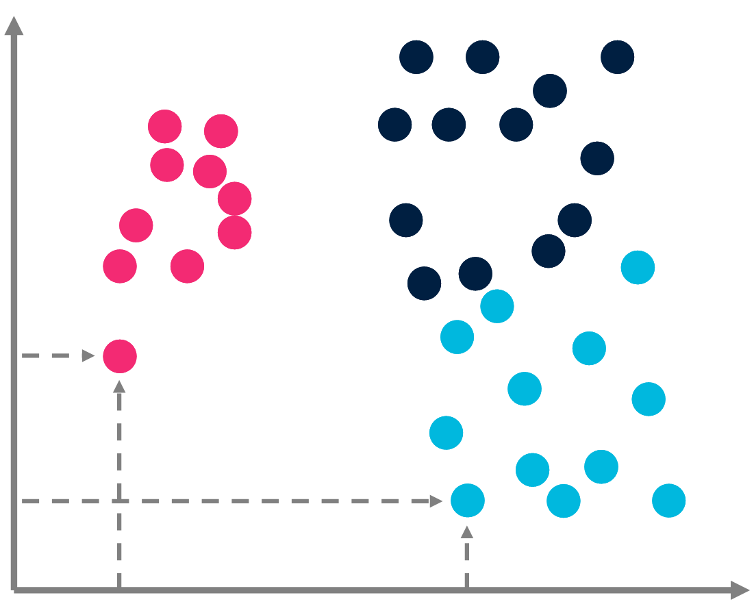
The problem is to associate a label (e.g. blue/red/dark) to each data point.Prototype-based models are routinely used for this. In doing so, they offer a compressed version of the classification.
 Classification
In a classification task, we consider a dataset \(X\) of \(|X|\) points \(x_j\). Each \(x_j\) is supposed to belong to a class labelled as \(y_j\). The problem is to learn which label \(y_j\) taken from the set of labels \(Y\) corresponds to \(x_j\).
The complexity of the classification is bounded by the amount of information required by rote learning.
$$C(\{(x_j, y_j)\} | X) \leq \sum_j C(\{y_j\}) \approx \sum_j |X| \times \log(|Y|)$$
 Classification
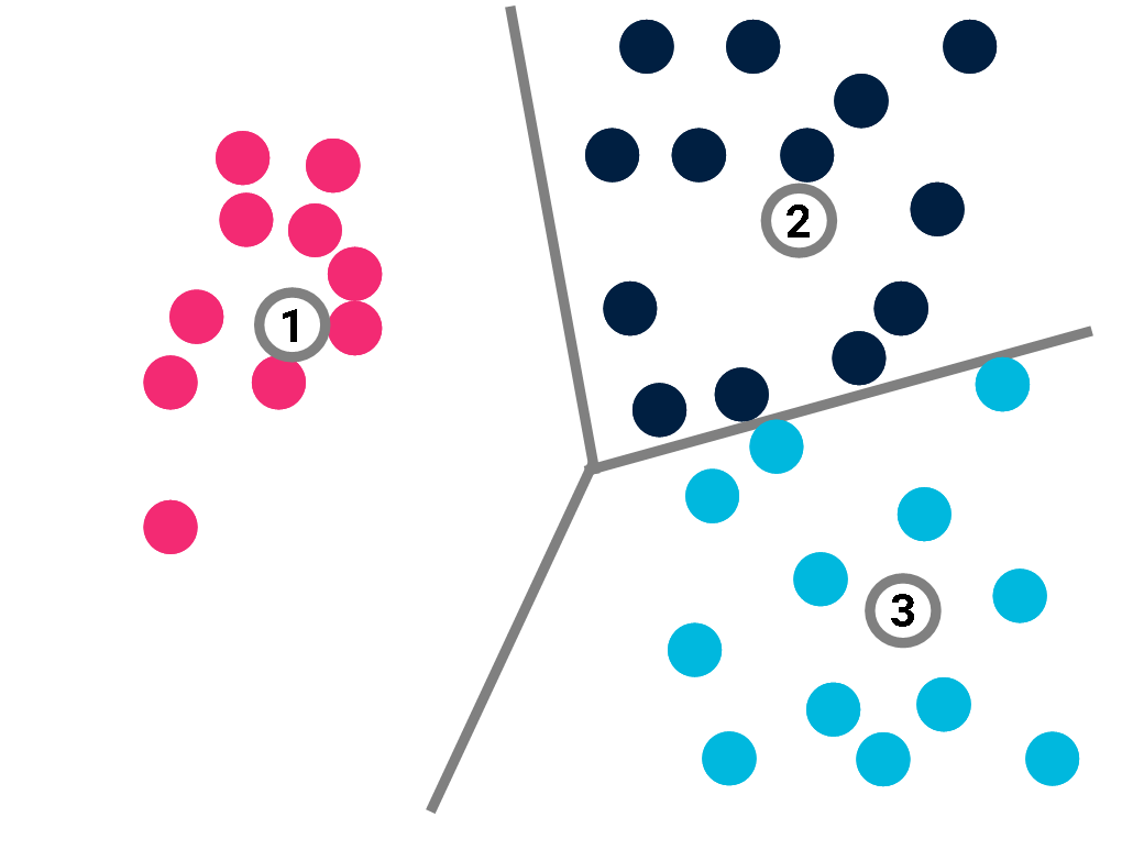
A prototype-based model \(\mathcal{M}\) would deduce the label of all points from those of its \(K\) prototypes \(\{p_k\}\), in the hope that:
$$\beta(x_i) = y_i$$
 Classification
A prototype-based model \(\mathcal{M}\) would deduce the label of all points from those of its \(K\) prototypes \(\{p_k\}\), in the hope that:
$$\beta(x_i) = y_i$$
The decision function \(\beta\) just returns the label of the closest prototype.
For instance, if the point is closer to prototype 3 (labeled "blue") than to any other prototype, the decision function will return "blue".
Classification
The complexity of the model is given by the complexity of its prototypes and their labels:
$$C(\mathcal{M}) \leq \sum_k C(p_k) + K \times \log (|Y|).$$
Now:
$$C(\{(x_j, y_j)\} | X) \leq C(\mathcal{M}) + \sum_{i,j} {C((x_j, y_j)} | X, \mathcal{M})$$
Since the decision function \(\beta\) is just a loop over the prototypes,
\(C((x_j, y_j) | X, \mathcal{M}) = 0\). So \(C(\{(x_j, y_j)\} | X)\) is found to be much smaller if \(K \ll |X|\) than if we only rely on rote learning.
Classification
The complexity of the model is given by the complexity of its prototypes and their labels:
$$C(\mathcal{M}) \leq \sum_k C(p_k) + K \times \log (|Y|).$$
Now:
$$C(\{(x_j, y_j)\} | X) \leq C(\mathcal{M}) \ll \sum_j |X| \times \log(|Y|)$$
We just have to remember the prototypes and their label to retrieve all labels, hence the compression.
Classification
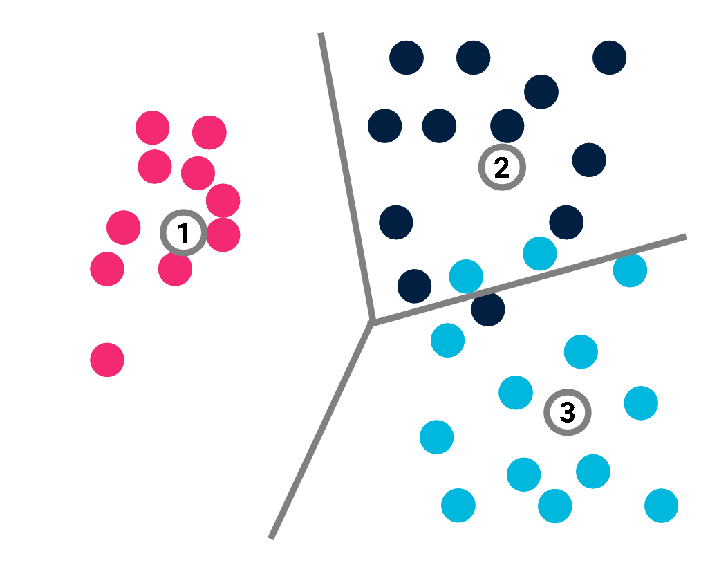
This is only true, however, if the model \(\mathcal{M}\) is perfect.
 Classification
This is only true, however, if the model \(\mathcal{M}\) is perfect.If not:
\(C((x_j, y_j) | X, \mathcal{M}) \neq 0\).
For each misclassified point, we may just specify its index the correct value of its label.
$$C(\{(x_j, y_j)\} | X, \mathcal{M}) \leq \sum_{i=1}^{|X|} (C(i) + C(y_i)) \times \mathbb{I}(y_i \neq \beta(x_i))$$
where \(\mathbb{I}\) is a function that converts a Boolean value into 0 or 1.
Classification
This is only true, however, if the model \(\mathcal{M}\) is perfect.If not:
\(C((x_j, y_j) | X, \mathcal{M}) \neq 0\).More simply, if there are \(n\) misclassified points, we get:
$$\sum_{i,j} C((x_j, y_j) | X, \mathcal{M}) \leq n \times (\log(|X|) +\log(|Y|)).$$
Classification To sum up:
$$C(\{(x_j, y_j)\} | X) \leq \sum_k C(p_k) + K \times \log (|Y|) + n \times (\log(|X|) +\log(|Y|))$$
If \(n\) is small, this may still represent a huge compression as compared to rote learning.
The right-hand side of this inequality can be used as a loss-function to determine the best prototype-based classification.