
	Telecom Paris Dep. Informatique & Réseaux Nils Holzenberger ← Home page February 2024

3EL05: Algorithmic Information and A.I.

Lecturer: Nils Holzenberger

Measuring Information through compression

What you will learn in this chapter:

How to compute complexity through compression
How to compare algorithmic information with Shannon’s information
How to detect languages through joint compression
How to use the Web to compute meaning similarity

Information as compression

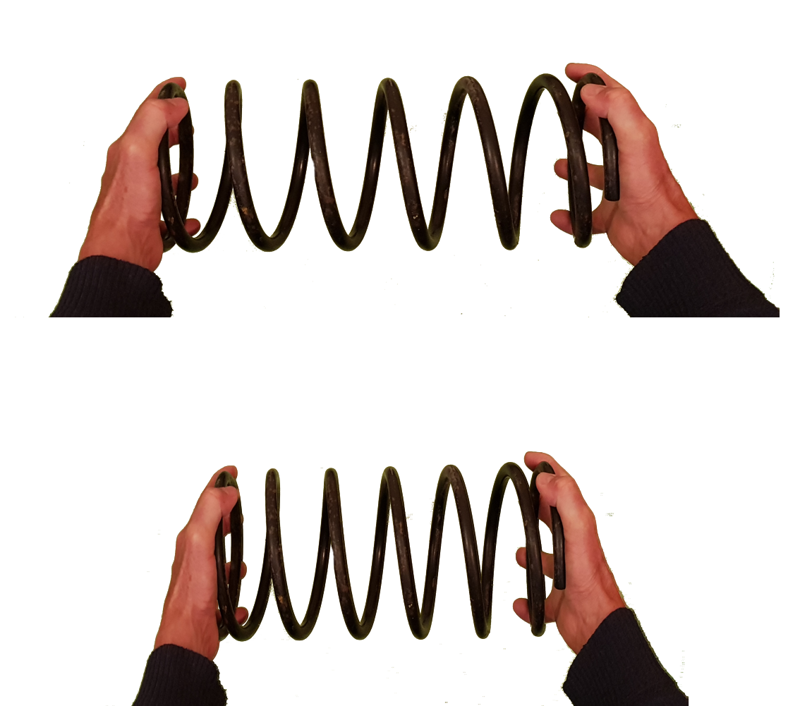
Problem: Can we define the quantity of information contained in a single, isolated object?

Information is what is left when any redundancy has been removed. Kolmogorov complexity does exactly that: It removes redundancy by performing ideal compression (without loss). The output represents the irreducible information contained in the object.

Compressing binary strings

Problem: Can we compress everything, and how much?

Understanding Artificial Intelligence
through Algorithmic Information Theory

Shrinking objects

aiai.telecom-paris.fr

How much can objects be compressed?

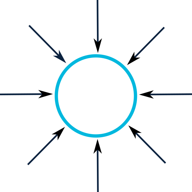Information is what is left after maximal compression.

How far can a given object be compressed?

Can we compress all objects?

How much can objects be compressed?

For the kind of objects that can be stored on a computer, such as videos, file sizes give us a hint.

For instance, a three-minute video such as this one weighs 70 MB in mkv format.

How much can objects be compressed?

Appearances may be deceptive, though.

This video has been generated by a 4 kB program! So a shrinking ratio of 17 000 to one.

This video won the Breakpoint PC 4K Intro competition in 2009. If you are aware of what 4 KB means, and if you watch the video, you can only be amazed. It is an example of what is called a demoscene.

Whenever an object can be compressed
down to a small description,
we know that there is not much information in it.

Let’s consider these three sequences.
(a) 1100110011001100110011001100110011001100110011001100
(b) 1001001000011111101101010100010001000010110100011000
(c) 0010100101110110101101000101101011011010001011001011

Sequence (a) is obviously simple. It can be described concisely.
In python: '1100' * 13.
This program can be seen as a compressed version of (a), since (a) can be recovered from it.

Sequence (b) is an attempt to write down ‘random’ binary digits by hand.
There seems to be no easy way to compress it.

Sequences (c) seems complex at first sight.
But an informed observer would know that sequence (c) represents the first digits of π in binary representation.
So (c) and any longer version of it can be compressed down to any short program that generates π.

    def pi(N):
        PiDividedByFour = 0
        for i in range(N):
            PiDividedByFour += (–1)**i /float(2*i+1)
        return 4* PiDividedByFour

It seems that many sequences can be compressed, or shrunk, down to a short description that captures their information content.

Really?


000000000000 000000000001 000000000010 000000000011 000000000100 . . . 111111111110 111111111111

Consider all binary sequences of size N. There are 2^N of them. For instance, there are 4096 binary sequences of length N = 12.

Some of these strings, such as the first and the last ones, are highly compressible.

For instance, we can represent the last one as '1' * N, and this can be coded with log₂(N) + O(1) bits, which is much less than N if N is not too small.

How many of these N-long sequences can be shrunk?


000000000000 000000000001 000000000010 000000000011 000000000100 . . . 111111111110 111111111111

Suppose we use a compressing program to compress the binary sequences of size N.

How many of them, at most, can be compressed by exactly k bits (k < N)?


000000000000 000000000001 000000000010 000000000011 000000000100 . . . 111111111110 111111111111

A sequence of N bits that is compressed by exactly k bits must be represented using N-k bits.

N-k bits can represent only 2^N-k different sequences. Since we want compression to be reversible, only 2^N-k sequences of length N at most can be compressed by exactly k bits.


000000000000 000000000001 000000000010 000000000011 000000000100 . . . 111111111110 111111111111

If we count all sequences of size $N$ that are possibly compressible by at least $k$ bits, we get:

$\sum\limits_{i=k}^{N} 2^{N-i} = \sum\limits_{j=0}^{N-k} 2^{j} = 2^{N-k+1} - 1$

Compared with $2^N$, this makes a proportion of roughly $\frac{2^{N-k+1}}{2^N} = 1/2^{k-1}$.
This means that only a tiny proportion of sequences may be compressed by at least k bits as soon as k is significant.

In other words, there is no miracle.
Shrinking has its limits.

If one considers all possible objects
(here, binary strings),
compression can spare you a lot of bits on some of them, but
these compressible objects are rare.

*Compressibility (1)*
What is the proportion, among all binary sequences of size 128, that can be compressed down to 100 bits or less?

*Compressibility (2)*
Consider a given compression method $Z$. Are there binary sequences of size $N$ that cannot be compressed through $Z$? (Hint: count the number of sequences that can be compressed by at least 1 bit.)

Zipping sequences

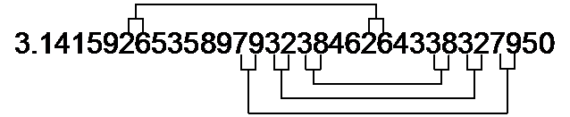Problem: How can we compress objects in practice?

Computer science offers a variety of tools to compress objects, such as the "jpeg" and "png" formats for images; for text or data files, one would use "zip", "bzip2" or "zpaq". The most basic mechanism at work in compressing programs consists of detecting duplicates in the sequence to be compressed.

Question: Does any duplicate pattern give rise to compression?

Answer: No. The pattern has to be long enough and the two copies should not be located too far apart.

Can we quantify these conditions?

The program CopyDetection.py is able to detect copies within a binary sequence. For instance, it may spot the pattern 0110111001101 of length L = 13 at two different locations of the following string:

When the program finds that a sequence of size L appears at location P₁ and again at location P₂, it refers to the first occurrence instead of repeating the pattern. The second occurrence of 0110111001101 in the above sequence is replaced by 1 1100 1101 where:

1 signals the code change,
1100 (= 12 in standard binary coding) signals that the original pattern ended 12 bits before (it is smarter to locate the end of the previous occurrence), and
1101 means that this initial pattern was 13 bits long.

Our code is using space delimiters, as in the Morse code (see Chapter 1).

$ CopyDetection.py 000101 0110111001101 000010111110 0110111001101 10010001011100110001
Original: 0001010110111001101000010111110011011100110110010001011100110001 - length: 64
Encoded: 0001010110111001101000010111110 1 1100 1101 10010001011100110001 - length: 60
Decoded: 0001010110111001101000010111110011011100110110010001011100110001 - Correct

(for convenience, the program’s arguments are joined into a single string).
Note one more time that as explained in Chapter 1, we do not count space characters when computing code length (this choice will be discussed in Chapter 3).

*Copy detection (1)*
Use the program CopyDetection.py to compress the sequence: 1110011010100111000110011100001101110100100011000101100000100011110000101100111011010011000001100011 What is the encoded version of the string?

Decimal to binary converter:

When given no argument, the program CopyDetection.py is applied to a pseudo-random binary string of size 100. Make several tries. You should be able to verify that pseudo-random sequences exhibit repeated patterns and thus are, slightly, compressible.

*Copy detection (2)*
Compute the largest distance between two repeats for which it is advantageous to code the repetition, if the repeated pattern is 0110111001101. Hint: you have to compute the distance between the onset (=beginning) of the two strings, so don’t forget to take the length of the pattern into account.

In what follows, $\log_{2+}$ means that the logarithm is rounded to the upper integer.
We approximate the complexity of an integer $n$ as $\log_{2+}(n+1)$.

*Copy detection (3)*
What is the theoretical condition on $L$ (length of the repeated pattern), $P_1$ (location of the 1^st occurrence) and $P_2$ (location of the 2^nd occurrence) to get compression with such a copy detection program? The constant $c$ represents the offset of the coding scheme (the extra heading 1 in the CopyDetection.py program).

Suggestion: Consider a way of compressing a sequence in which the same pattern occurs 3 times or more.

Information as absence of redundancy

Problem: Does compression measure redundancy?

Redundancy obviously does not contribute to information. This is why compression is the best tool to measure information. For instance, unbalanced binary sequences that have more 0s than 1s, or more 1s than 0s, are highly redundant.

000000000100010000000000000001000001010000000000000000000000010100000000001000000000000000000

They are expected to be compressible. Can we verify that?

The program BinSeqGenerator.py computes compression factors for biased sequences, using Zip (averaged over several trials; 100% compression corresponds here to the compression of a constant string).
For instance, if you execute: BinSeqGenerator.py 1000 33
the program generates 1000-bit long sequences with 33% of 1s and tries to zip them.

*Biased sequence (1)*
What average compression factor do you get for strings of length 1000 with a 22% bias?

Information: Complexity vs. frequency

Algorithmic information and Shannon’s information

Problem: What is the link between Algorithmic Information and Shannon’s information?

Huffman codes

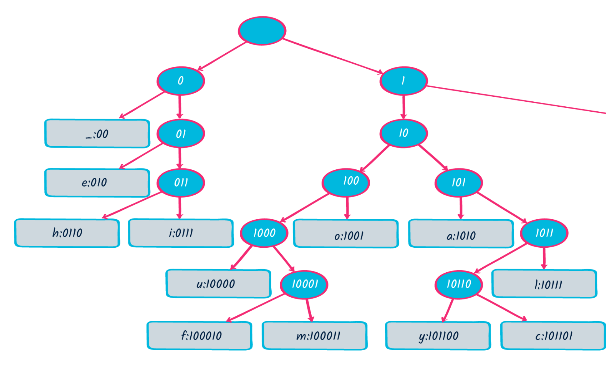Problem: How can we take advantage of unbalanced statistics to compress information?

When symbols are repeated (as in digital communications) and frequencies are available, Shannon’s theory of information tells us that maximal compression on average can be achieved through variable-length codes. For instance, if you want to represent English texts in a compact binary code, you should choose a shorter code for ‘E’ than for ‘Z’. Huffman codes do this optimally.

You can generate a Huffman code online.

I’m not sure whether Shannon’s information and Algorithmic information measure the same thing.		You mean that they would be equivalent?

I know they are not.		Yes, because Algorithmic information is about single objects.

Ah! Oh yes, you’re right. Shannon’s information is about events.		Or rather, about occurrences of repeated events.

That’s why Shannon relies on the probability of events.		And probabilities do not always apply. What’s the probability of π?

And yet, when probabilities make sense, both notions are equivalent.		I’m not even sure of that.

Why?		Because complexity is a minimum over all computations. And it may change through time.

You mean, it may depend on the context?		Yes. A second occurrence of an event just requires a mere copy. It’s simple.

And yet, this second occurrence might be surprising if the event is rare. So it should carry much information.		Yes. It was not totally clear to me. So I asked the teachers.

And...?		I’ve been told that all this would become clear when we define algorithmic probability in Chapter 3.

That’s funny. Me, I’ve been told that I would understand all this in Chapter 5, when we talk about subjective information.		Ok, let’s wait and see...

Inferring complexity from Web data

Problem: Is there a link between complexity and Web frequency?

As we saw, some integers, such as round numbers, are simpler than others. Does it affect their frequency on the Web? The picture below represents the number of hits (in 2009) declared by Yahoo and Google for requests consisting of numbers between 1000 and 2050 (the correlation for both search engines is 0.98; note the logarithmic vertical scale).


	More recent version

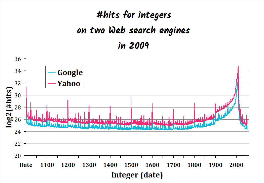
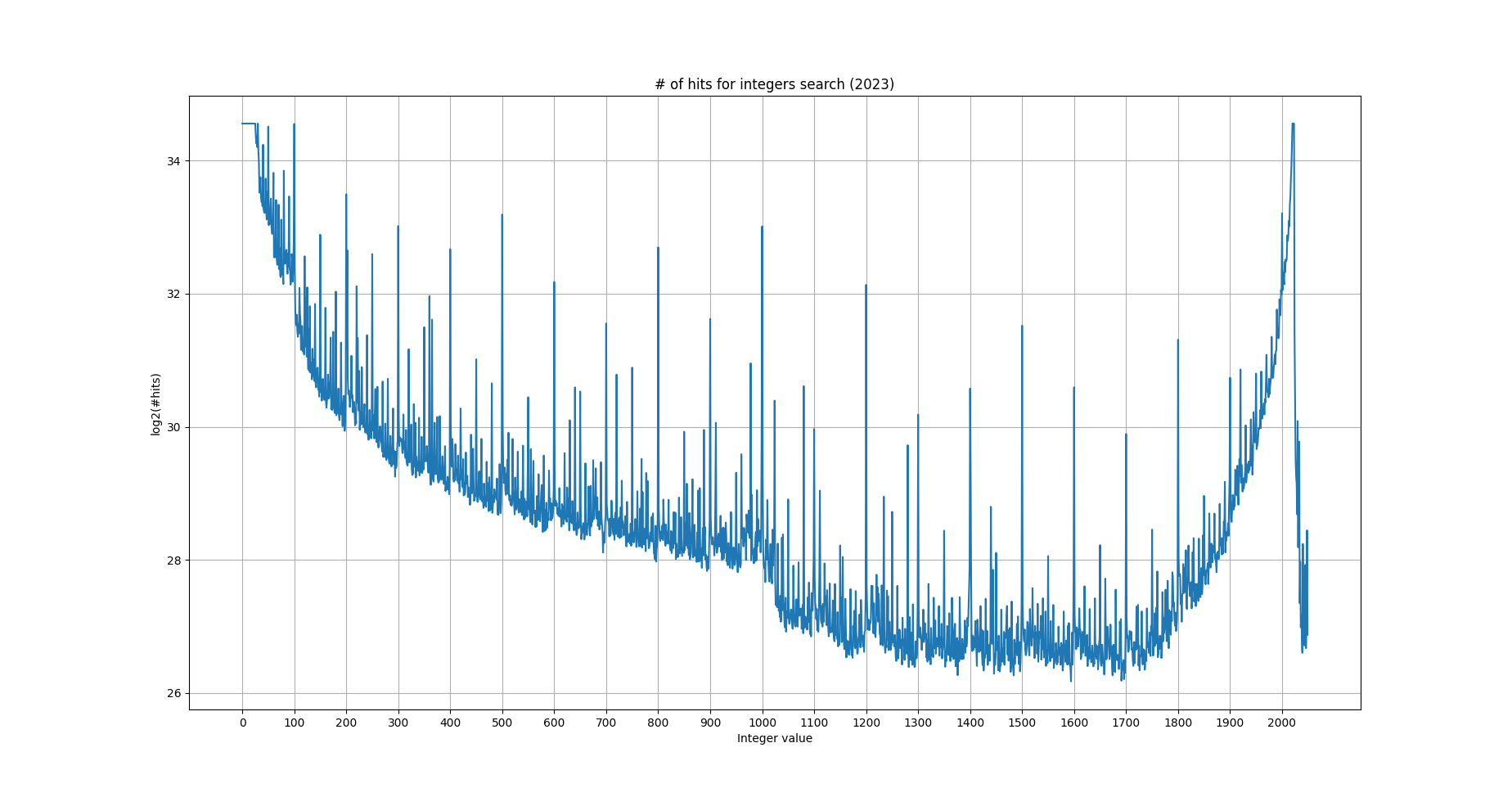
One can unambiguously see that larger frequencies in the Web correspond to "simple" numbers:

Multiples of 100
1024
Multiples of 50
Recent dates

Question: stallion is more complex (and less frequent) than horse. What about quadruped?

Answer: quadruped is indeed less frequent than horse. The point is that quadruped is more complex a concept than horse, even if a horse is a quadruped with additional characteristics (just ask children about horses and quadrupeds).

Some authors suggested the possibility of inverting the relation between complexity and frequency. The frequency of words in texts can be assessed using a search engine. Though it is difficult to infer the real number of pages indexed by search engines, it seems that dividing Google’s declared number of hits by 2 × 10¹² gives a reasonable estimate of actual frequency. For instance, the word "spoon" can be considered to occur with a frequency of 0.02%, whereas the frequency of "book" is 0.87%.

If a word w occurs with a frequency f, we get an estimate of the complexity K(w) of the corresponding concept through the formula:

K(w) ≲ log(1/f).

This formula, which holds up to an additional constant, will be further explored in Chapter 3. It serves as the basis for the use of log(1/f) as an approximation of K(w).

Zipf’s law

Problem: Zipf’s law describes a spectacular phenomenon. Where does it come from?

Understanding Artificial Intelligence
through Algorithmic Information Theory

Zipf’s law

aiai.telecom-paris.fr

Zipf’s law describes an absolutely remarkable and quite unexpected phenomenon.

It links the frequency of words to their rank by frequency.

The law was first discovered in 1928 by Edward Condon

and then by George Zipf.

What does the "Condon-Zipf law" say?

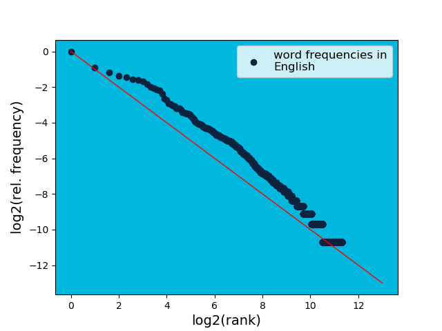Zipf’s law: $r_f(w) \approx \frac{k}{f(w)}$

or: $log(f(w)) \approx -log(r_f(w)) + c$

$ f(w) $ is the frequency of the word $ w $ in the language, $ r_f(w) $ is the rank of $ w $ in the vocabulary sorted by frequency and $ c $ is a constant.

Zipf’s law: $r_f(w) \approx \frac{k}{f(w)}$

or: $log(f(w)) \approx -log(r_f(w)) + c$

This means that the 10^th most frequent word is 10 times more frequent than the 100^th most frequent word, which is itself 10 times more frequent than the 1000^th most frequent word, which is itself 10 times more frequent than the 10 000^th most frequent word, and so on. Or the 10^th most frequent word is twice more frequent than the 20^th most frequent word, 4 times more frequent than the 40^th most frequent word, 8 times more frequent than the 80^th most frequent word, and so on.

Why is it so?

Zipf’s law: $r_f(w) \approx \frac{k}{f(w)}$

or: $log(f(w)) \approx -log(r_f(w)) + c$

This plot has been drawn based on the frequency of words in Alice’s adventures in Wonderland.
Several similar plots are available in this compressed file (look into texts/_Zipf). Yes, it works for Chinese too!
You may try on any corpus in any language you may choose using this small program.

Zipf’s law: $r_f(w) \approx \frac{k}{f(w)}$

or: $log(f(w)) \approx -log(r_f(w)) + c$

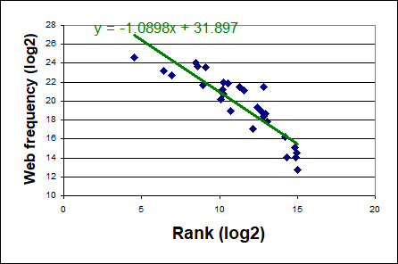
If we plot the number of hits of a few words in a search engine against their frequency rank in the language, we get a linear tendency in log-log coordinates.
This conformity with Zipf’s law suggests that the Web, as seen through search engines, offers an accurate image of language use.

The data displayed above are available in this table
(format .xls, format .csv).

Word frequency ranks can be found in various Websites, such as this one, or this one or this one.

Suggestions

Study the Heaps-Herdan law (the log-log linear dependence of corpus size and vocabulary size).

Zipf’s law and Kolmogorov complexity

Zipf’s law is an empirical phenomenon. It is not easy to explain.

In 1936, George K. Zipf supposed that the frequency of words in language results from the strategy used by people during their mental search through the vocabulary to find appropriate words to express intended meanings. As a consequence, one may suppose that words are stored by decreasing frequency in our minds.

If so, Kolmogorov complexity may explain Zipf’s law.

On the one hand, the complexity of words is related to their frequency of use, through the formula: K(s) ≈ log(1/f) + c.
On the other hand, the complexity of words can be inferred from their rank in the vocabulary: K(s) = log(1/r) + c.

This way, Kolmogorov complexity can be seen as acting as a go-between which links rank to frequency.

*Zipf law*
Let’s take two books of similar size, written in two different languages (we suppose they have no words in common). Will the concatenation of the two books verify Zipf’s law?

Suggestion: Use the program Zipf.py to verify Zipf’s law on your own corpus. See for example Frankenstein and Alice's Adventures in Wonderland on Project Gutenberg.

Using AIT to detect similarity

Problem: Can we measure shared information using compression?

AIT principles, implemented through compression, are used in a variety of practical applications: rediscover language genealogy without knowing linguistics, attributing authorship without knowing authors’ styles, determining concept similarity without any knowledge of semantics, finding out Coronavirus-19 phylogeny while ignoring biological knowledge, and more. We explore some of these techniques now.

Detecting language through compression

Understanding Artificial Intelligence
through Algorithmic Information Theory

Detecting Language Proximity through Compression

aiai.telecom-paris.fr

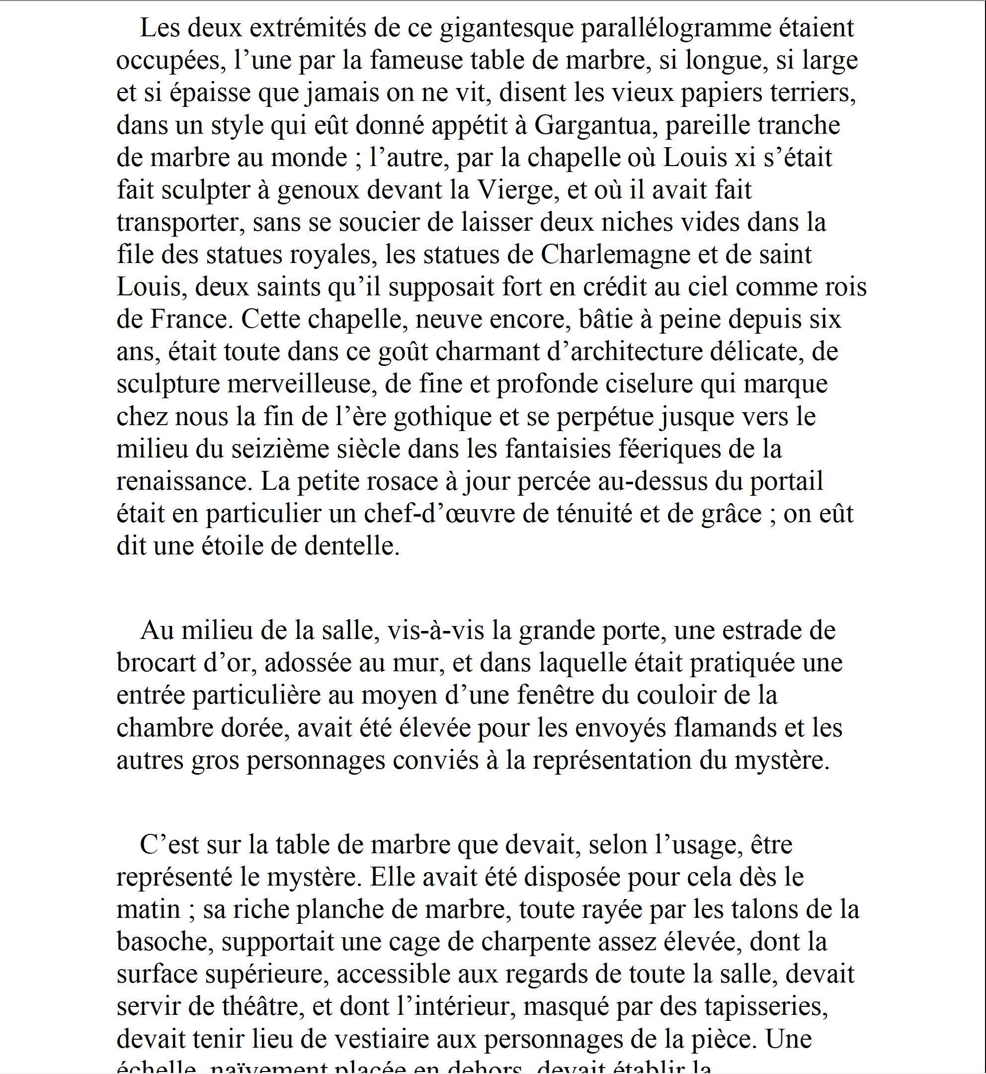
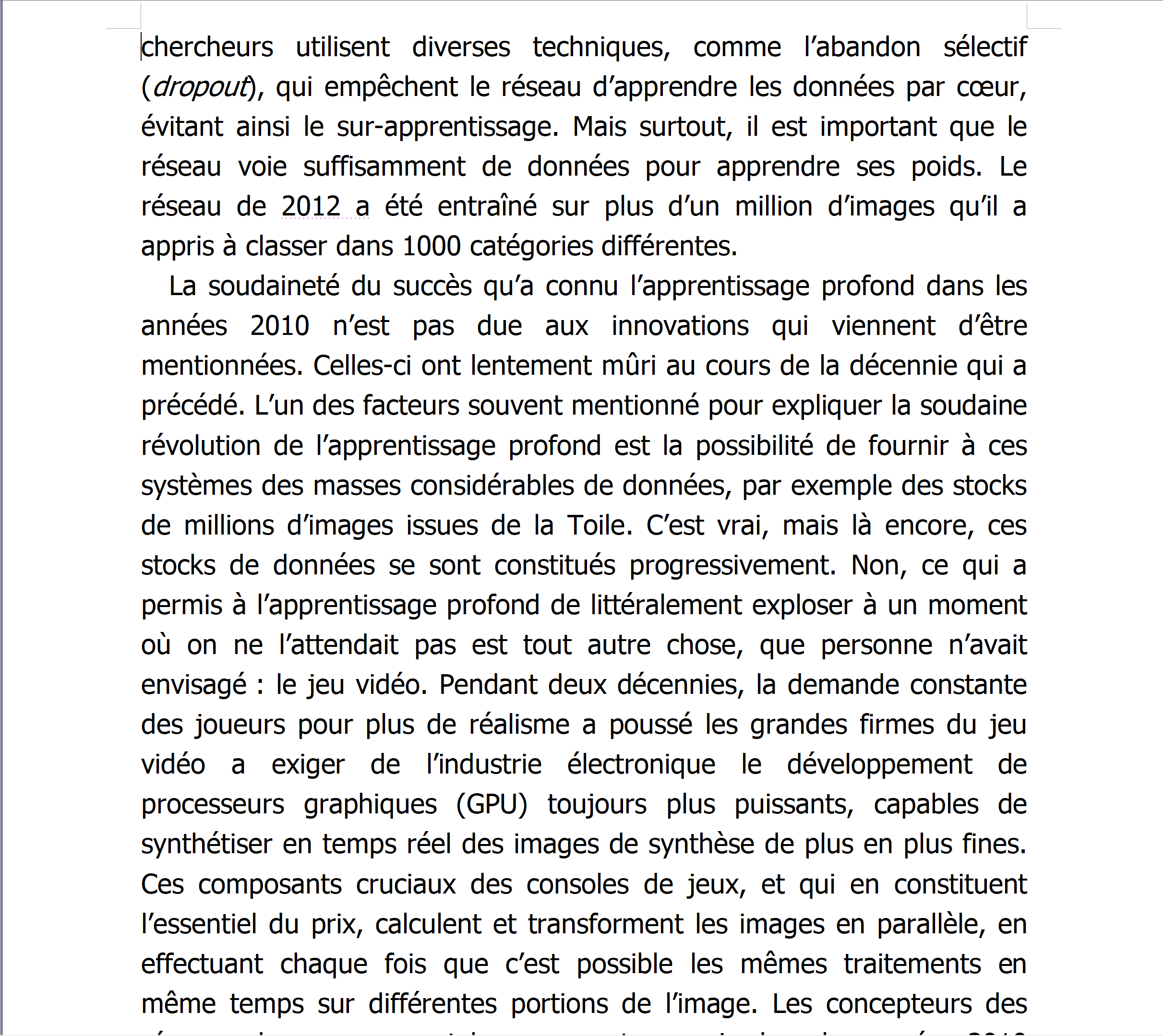Intuitively, two texts T₁ and T₂, considered as mere strings, should share more information if they are written in the same language than when compared with a third text T₃ written in a different language.

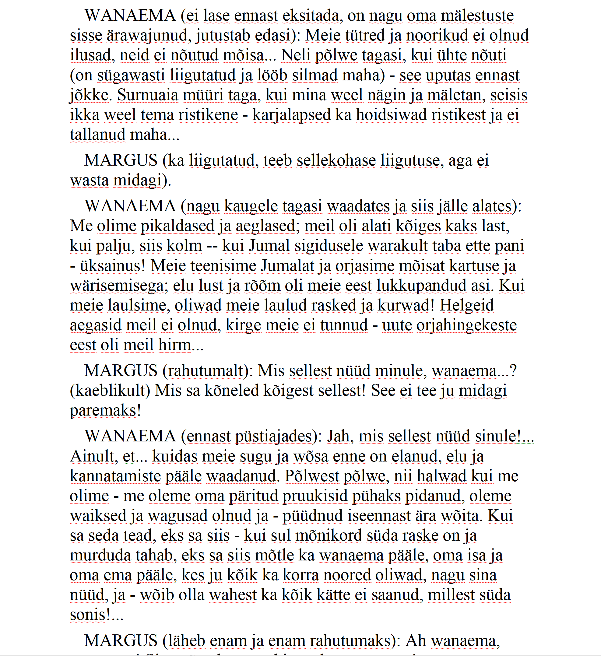This is due to the greater redundancy if X and Y share many words.
Conditional complexity is the most natural way to measure information sharing. We expect:

C(T₁ | T₂) << C(T₁ | T₃)

For practical purposes, compression can be used as a proxy for complexity.
Using the Chain Rule, we can write:

C(T₁ | T₂) > C(T₁, T₂) – C(T₂)

Measuring the output of compressor Z as proxy for C and text concatenation instead of conjunction, we can estimate C(T₁ | T₂) by:

length(Z(T₁ + T₂)) – length(Z(T₂))

This measure of conditional complexity through joint compression may be used to represent the resemblance between objects such as texts.

length(Z(T₁ + T₂)) – length(Z(T₂))

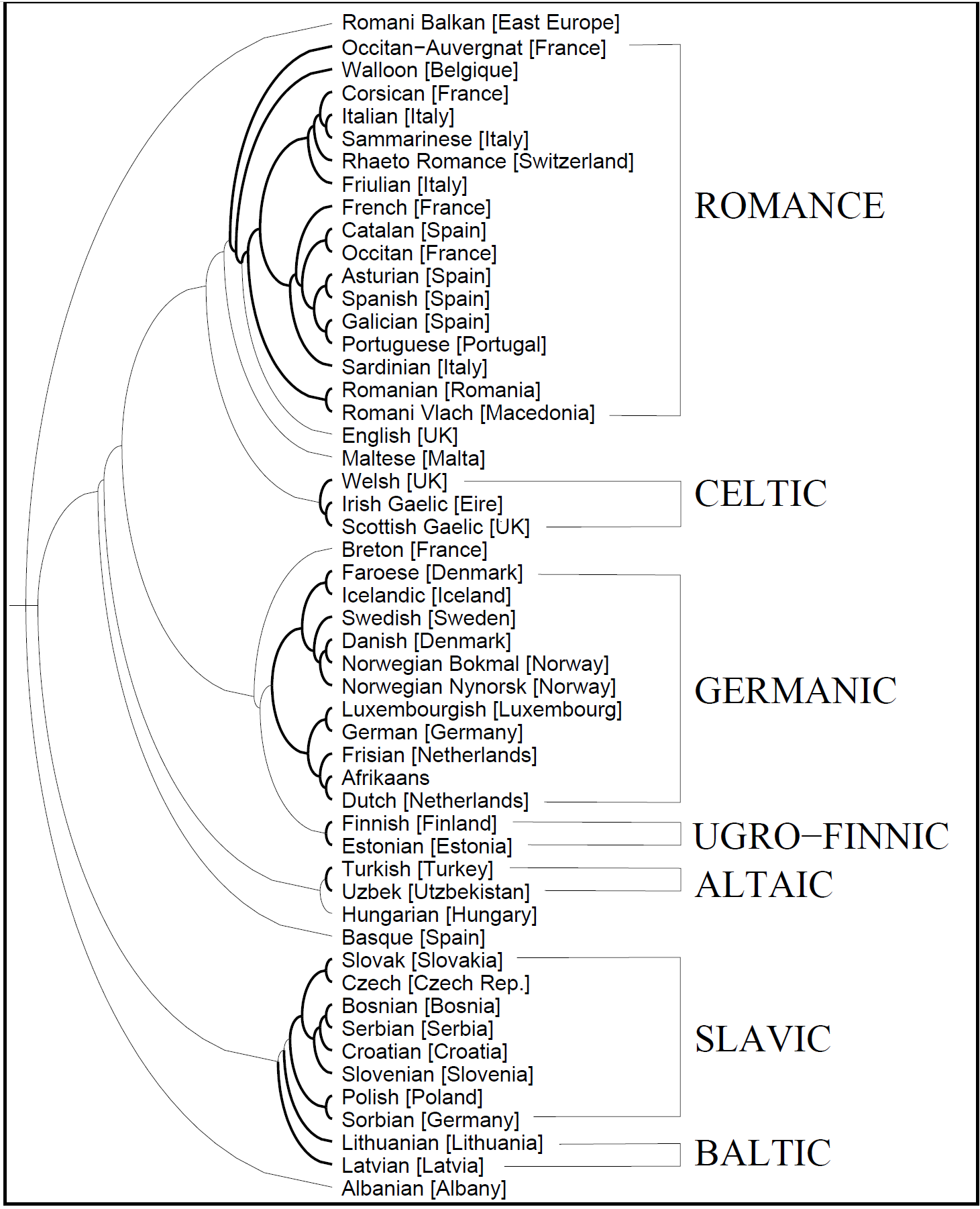In 2002, three scientists, Dario Benedetto, Emanuele Caglioti and Vittorio Loreto, were able to measure language proximity using a mere compressor such as Zip.

The language tree they could reconstruct with this estimate of conditional complexity matches the main language families that linguists stepwise developed during a century!
You might notice a couple of miclassifications, though.

Let’s consider a set of reference texts T_i written in different languages. Such texts can be found in texts.zip. They have been stored in utf-8 format.
Then you may build a small text X (typically one-page long) in whatever language you want. This text will be used as a probe. You may cut-and-paste some text into your editor before saving it as X (instead of saving it directly from the browser) to eliminate html tags and links. Be sure it’s saved in utf-8 format.

We want to see if joint compression with the T_is can identify X’s language. To do so, we rank the T_i by increasing values of:

length(Z(T_i + X)) – length(Z(T_i))

where Z is your favourite compressor. It would be great if the T_i that comes first correctly identifies the language (or the author) of X.

Use the program TextDistance.py to compute length(Z(T_i + YourText)) – length(Z(T_i)), where the T_i are the texts in various languages (make sure that YourText is small as compared to T_i). Note: this program imports NumberCompression.py.

Suggestion: One may try to use the same technique for automatic authorship attribution. Various texts can be found online for famous authors, such as (Zola, Hugo and Sand).

NID: A universal distance

Problem: Can we define a concept similarity measure based on Algorithmic Information?

Complexity offers a natural measure of concept similarity. We may use conditional complexity K(x|y) to estimate how much x differs from y.
We can turn this measure into an operational method by estimating K using Web frequencies, as we did previously.

Suppose you want to measure the conditional complexity K(rider | horse) between two concepts, rider and horse. You can get an estimate by computing log(1/f(rider | horse)). Conditional frequency f(rider | horse) can be computed the same way as conditional probability: f(rider | horse) = f(rider+horse)/f(horse).

Let’s perform some measures on a Web search engine:
- "rider" gets 74 × 10⁶ hits on Bing,
- "horse" gets 72.5 × 10⁶,
- "rider + horse" gets 13 × 10⁶.
The conditional frequency, according to Bing, is therefore f(rider | horse) = 13/72.5 = 0.18, and the conditional complexity K(rider | horse) = 2.47 bits.
By contrast, f(rider | the) = 71/13300 = 0.005 ≈ f(rider), and so K(rider | the) ≈ K(rider).
This makes sense: in a context in which "horse" has been mentioned, "rider" is less complex than in a context in which "the" has been mentioned (which amounts to no context at all).

Question: Conditional complexity is asymmetrical. Can we define a genuine distance based on it?

Answer: Yes, and this is what Paul Vitányi and his colleagues did in 2004 by defining the "Normalized Information distance" (NID).

Understanding Artificial Intelligence
through Algorithmic Information Theory

NID:
A "universal" distance

aiai.telecom-paris.fr

In 1998, Charles Bennett and his colleagues introduced
the Normalized Information Distance (NID).

NID is a universal distance.

For any pair of objects, NID determines what is common to them, and only keeps their difference to measure the distance that separates them.

By doing so, NID can be regarded as "the most intelligent" distance!

NID is based on conditional complexity K(x|y).

Conditional complexity measures the amount of information contained in x that is not already present in y.

We’ll proceed from K(x|y) to NID(x,y) in three steps.

K(x|y)

Step 1: symmetry.

Let’s make conditional complexity symmetrical, by considering max[K(x|y), K(y|x)] instead of K(x|y).

This will measure the amount of information that is not shared between x and y.

max[K(x|y), K(y|x)]

Step 2: normalization.

Suppose that two objects differ by n bits of information.

If n is significant compared to their complexity, then they are very different.

However, if the objects are complex and now the same n bits represent a small amount compared to their complexity, then the two objects are very similar.

max[K(x|y), K(y|x)]

Step 2: normalization.

To take this relative effect into account, let’s divide the similarity measure by the objects’ complexity. $$ \frac{max[K(x|y), K(y|x)]}{max[K(x), K(y)]} $$

$\frac{max[K(x|y), K(y|x)]}{max[K(x), K(y)]}$

Step 3: chain rule.

The Chain Rule for K says that (up to an additional constant, neglected here): K(x, y) < K(x|y) + K(y).

If we replace K(x|y) by K(x, y) – K(y) in the above expression, we get what Bennett and his colleagues defined as Normalized Information Distance, or NID. $$ NID(x, y) = \frac{K(x, y) - min[K(x), K(y)]}{max[K(x), K(y)]} $$

$NID(x, y) = \frac{K(x, y) - min[K(x), K(y)]}{max[K(x), K(y)]}$

This distance has values between 0 and 1. Unlike usual distances that rely on predetermined computations, NID discovers for each pair {x,y} what x and y have in common.

For this reason, NID may be considered as the "most itelligent" distance one may think of.

This means that if two objects x and y are close to each other according to any given computable distance, then x and y will be found close to each other by NID.

See (Li, Chen & Li, 2004) for details.

The Google distance

Problem: Can we infer concept similarity by measuring conditional complexity on the Web?

From NID to NCD. The Normalized Information Distance (NID) remains an abstract notion, based on Kolmogorov complexity. If we substitute a mere compressor such as "zip" for Kolmogorov Complexity, NID becomes NCD: the Normalized Compression Distance (here $Z$ designates the length of the compressor output):

$NCD(x, y) = \frac{Z(x, y) - min[Z(x), Z(y)]}{max[Z(x), Z(y)]}$

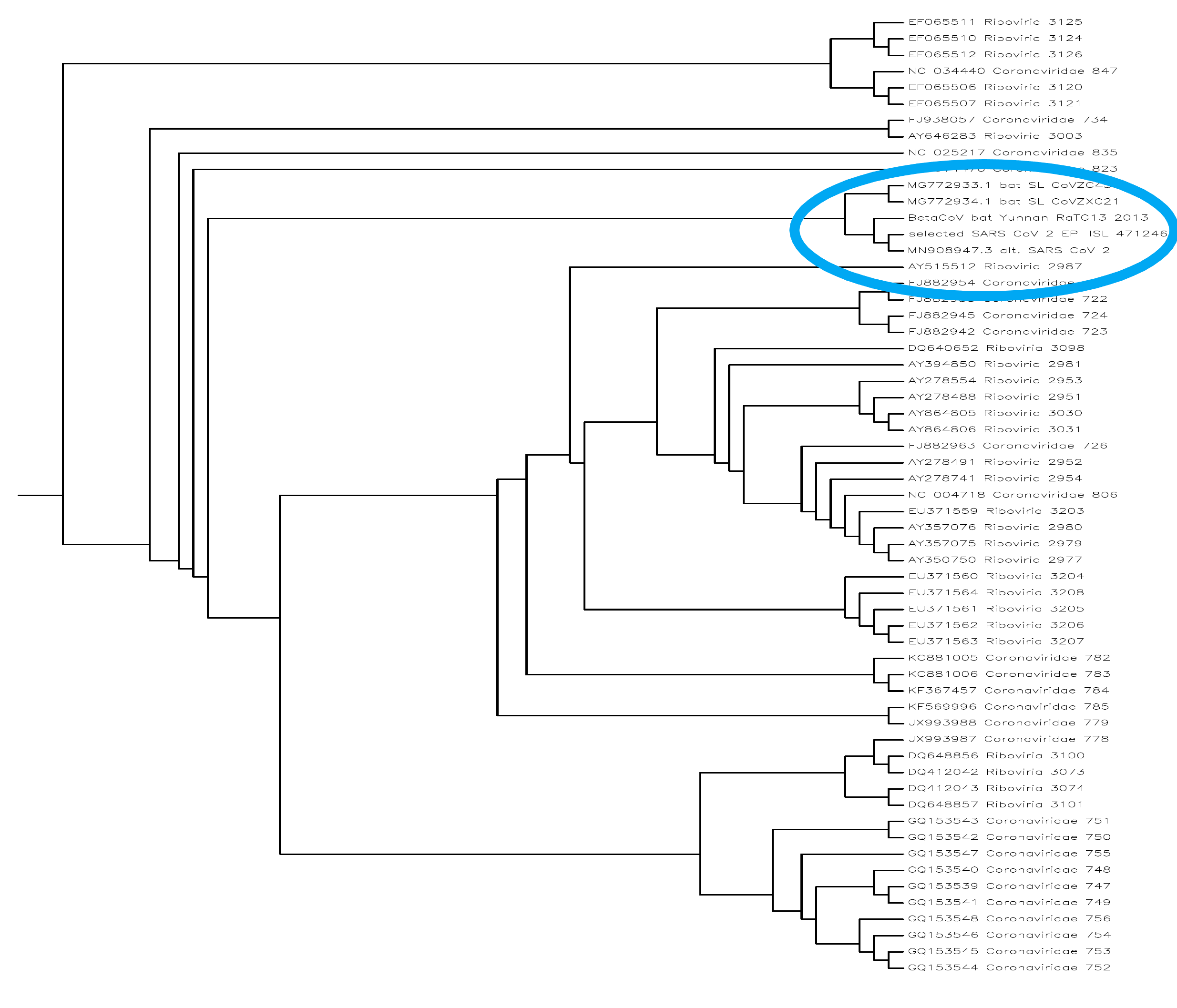
The advantage of NCD is that it is computable and can be used in practice.

NCD has been used to compute distances between languages or distances between species based on DNA strings (Li, Chen & Li, 2004), and more recently to determine the phylogeny of the SARS-COV2 virus (Vitanyi & Cilibrasi, 2020) (see figure).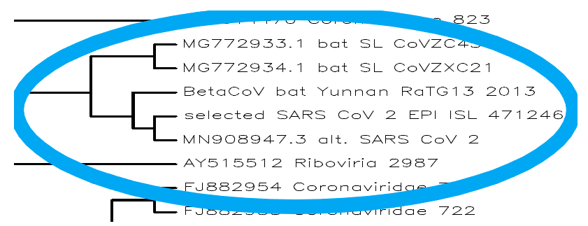

*NCD*
Consider this Python program and its execution. import os, zlib # Opening four sample texts SampleFiles = ['sample1.txt', 'sample2.txt', 'sample3.txt', 'sample4.txt'] Texts = [open(F, 'rb').read() for F in SampleFiles] # compressing texts ZSizes = [len(zlib.compress(T)) for T in Texts] print('Compressed sizes:\t', ZSizes) # co-compressing texts print('Z(sample1 + sample2):\t', len(zlib.compress(Texts[0] + Texts[1]))) print('Z(sample3 + sample4):\t', len(zlib.compress(Texts[2] + Texts[3]))) $ SampleCompress.py Compressed sizes: [8247, 10793, 2151, 2829] Z(sample1 + sample2): 18022 Z(sample3 + sample4): 4352 Which pair should be regarded as more similar according to NCD, and by how much?

Question: Can we go one step further and use the Web to define a complexity-based distance between concepts?

Answer: Yes, and this is what Rudi Cilibrasi and Paul Vitányi did in 2007 by creating what they call the "Google distance".

From NCD to the "Google distance". We may use Web data to estimate K. Let’s start from the expression of NID:

$NID(x, y) = \frac{K(x, y) - min[K(x), K(y)]}{max[K(x), K(y)]}$

As we did to get an estimate of conditional complexity, we may replace K(x) by log₂(1/f(x)), where f(x) is the observed frequency of x on the Web, or rather by log₂(N/g(x)), where N is the corresponding total number of indexed pages and g(x) denotes the number of pages containing x.

$NGD(x, y) = \frac{max[log(g(x)), log(g(y))] - log(g(x, y))}{log(N) - min[log(g(x)), log(g(y))]}$

NGD stands for Normalized Google Distance, after the name of the search engine used by Cilibrasi and Vitányi. $g(x, y)$ denotes the number of pages containing both $x$ and $y$, as reported by the Web search engine (for Google, it seems that N = 2 × 10¹² is a reasonable estimate, in relation to the declared number of hits).

Intuitively, NID is supposed to extract by whatever ideal means what is common to two objects. By estimating K using a Web search engine, as in NGD, the two objects are compared not through their common structural features, but through the human-created contexts in which they co-occur.

*NID-NCD-NGD*
Select all of the statements that are true.

Interview

Recap

Take-home message

We hope you enjoyed this chapter on AIT and compression.
Let’s leave the last word to Angel@ and Alexandr@.

We saw that most objects can’t be significantly compressed. That’s disturbing!		Why?

It means that AIT is concerned with only a small proportion of all possible objects.		So what? It just means that most objects are boring.

And so, you mean that an AI program should pay attention only to compressible objects?		Or only to objects that it is able to compress.

If I follow you correctly, Kolmogorov complexity can be used to measure intelligence.		??

Yes. Kolmogorov complexity is based on an ideal compressor. If making sense of data amounts to achieving compression, then KC offers an upper limit of what intelligent processing can do.		Ah, OK... I see. Personally, I felt more concerned by the practical side of it.

You mean, actual compression using Zip?		Not only. It’s nice to know that we can assess complexity through frequency measures.

Yes. It connects Kolmogorov complexity to Shannon’s information.		And using a search engine to compute semantic distance is really cool!

Ah, the story about the universal distance and the "Google distance"? Yes, nice! But my favorite is still the story about Zipf’s law.		Oh yes. Incredible, isn’t it? The law is so simple: F = k/r. And it applies to everything we write!

It seems to make sense, though. I mean, when you look at it in terms of minimal description.		Yes. It suggests that Kolmogorov complexity is not only a tool. It explains things.

Bibliography

Benedetto, D., Caglioti, E. & Loreto, V. (2002). Language trees and zipping. Physical Review Letters, 88 (48702).
Cilibrasi, R. & Vitányi, P. (2007). The Google similarity distance. IEEE Transactions on Knowledge and Data Engineering, 19 (3), 370-383.
Condon, E. U. (1928). Statistics of vocabulary. Science, 67 (1733), 300.
Li, M., Chen, X., Li, X., Ma, B. & Vitányi, P. (2004). The similarity metric. IEEE transactions on Information Theory, 50 (12), 3250-3264.
Vitanyi, P. & Cilibrasi, R. (2020). Phylogeny of the COVID-19 Virus SARS-CoV-2 by Compression. bioRxiv, 10.1101/2020.07.22.216242.
Zipf, G. K. (1936). The psycho-biology of language: An introduction to dynamic philology. Routledge.

Contents

Measuring Information through compression

Information as compression

Compressing binary strings

Zipping sequences

Information as absence of redundancy

Information: Complexity vs. frequency

Algorithmic information and Shannon’s information

Huffman codes

Inferring complexity from Web data

Zipf’s law

Zipf’s law and Kolmogorov complexity

Using AIT to detect similarity

Detecting language through compression

NID: A universal distance

The Google distance

Interview

Recap

Take-home message

Bibliography